Robots are revolutionizing industries by performing critical tasks in manufacturing, transportation, and inspection, significantly increasing production efficiency in sectors such as logistics and agriculture.

However, to truly unlock their potential, we face the dual challenge of ensuring the robots can efficiently perform their designated tasks while also minimizing the resources to design these robots, such as costs or power consumption. This balance is crucial for maintaining profitability and competitiveness.

This brings us to a pivotal question: how can we automate the design of these robots to ensure they are task-efficient and resource-efficient?

My research aims to address this challenge, paving the way for the next generation of smart, efficient, and economically viable mobile robots.

Designing mobile robots presents a variety of complex challenges. One major challenge is the integration of numerous interconnected components. Consider a Mars rover: it has six wheels, an arm, and multiple sensors for navigation and scientific measurements. Each component requires hardware and software that must work together. For instance, sensors and actuators need a power supply from the battery, and the software requires computational resources from a computing unit.

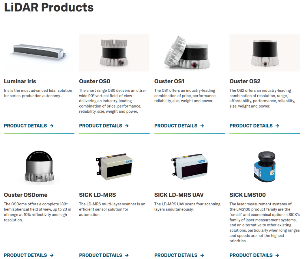
Another challenge is the overwhelming number of design options available. Most components, such as the choice of a lidar sensor for your robot, are typically off-the-shelf items from catalogs. Beyond selecting the right lidar, designers must also decide on sensor placement and the integration of other sensor types, such as cameras and radars. Additionally, decisions must be made regarding software and actuators.

Designing a robot also involves numerous trade-offs. For example, consider the various types of vacuum cleaning robots available for home use. These robots differ in functionalities, such as vacuum cleaning, wet cleaning, and battery life. The more functionalities a robot has, the higher the cost. My goal is to solve the design problem for a robot by ensuring it provides specific functionalities, such as cleaning a room with a certain area in square meters.

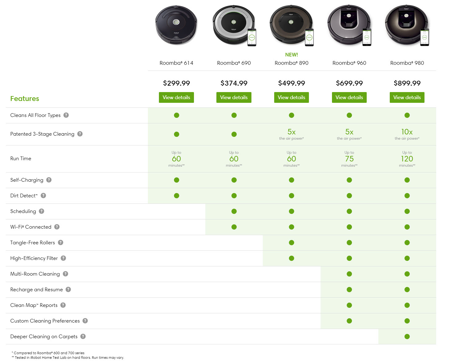
Achieving these functionalities requires resources such as cost and mass. The higher the performance required, the more resources are needed. For instance, cleaning a larger room requires a bigger, more expensive, and heavier battery. Therefore, my aim is to identify design choices, known as implementations, that provide the necessary functionalities while minimizing resource use, or that offer the best possible functionality within given resource constraints.

The following problem is addressed in the context of designing an autonomous vehicle. We begin by defining the task the robot must perform. Understanding the specific task is crucial for identifying a resource-efficient design.

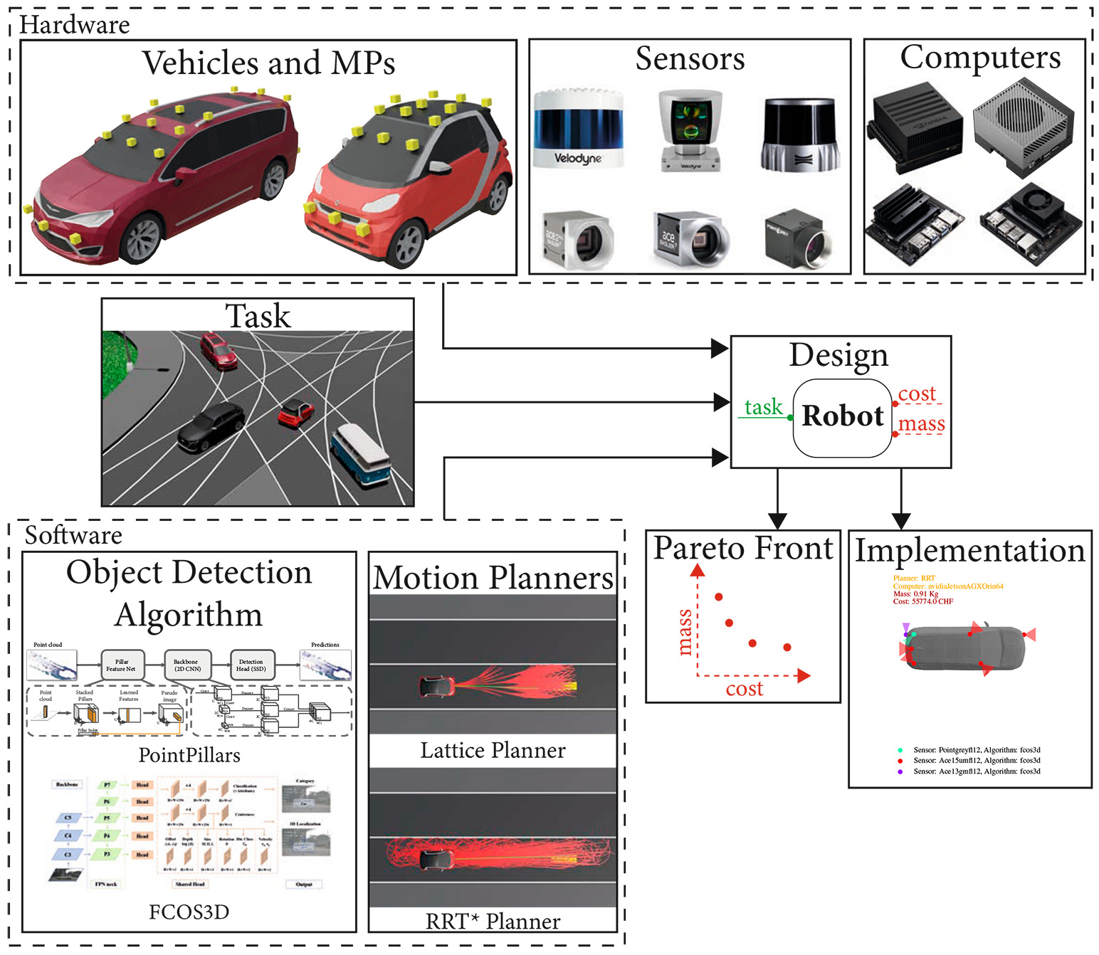
Next, we turn to a catalog of software options. On one hand, there are object detection algorithms that analyze sensor data, such as images or lidar point clouds, to detect objects such as cars and pedestrians. These perception algorithms, often based on deep neural networks, are crucial for enabling the vehicle to understand its environment. On the other hand, we have motion planners, which are responsible for calculating the robot's trajectories or actions to achieve its goals.

We also examine catalogs of hardware components, including vehicle bodies with predefined sensor mounting positions, a variety of sensors such as cameras and lidars, and computing units.

Our goal in using these catalogs is to identify a robot design that meets the task requirements while minimizing resource use. The final output, for example, could be a Pareto front of resources and their corresponding implementations. This enables us to visualize trade-offs and select the most efficient design.

Now, we embark on a critical aspect of our journey: understanding the perception requirements for autonomous agents. Perception is the cornerstone of a mobile robot's ability to navigate and interact with its environment. By determining the information needed by the motion planner, we can define the perception requirements for our system.

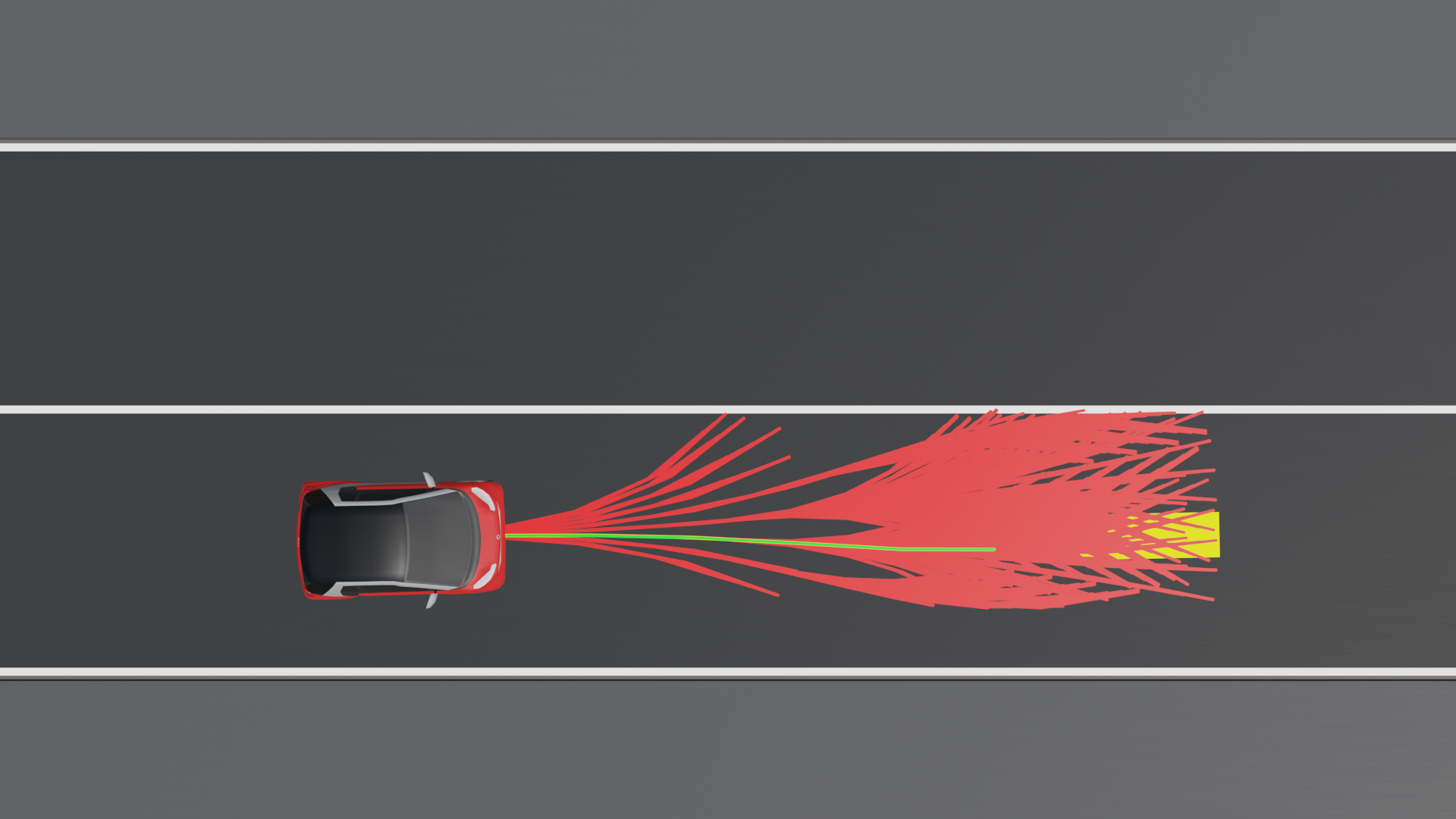
A specific type of motion planner is the sampling-based motion planner. These planners bypass the need for a mathematical representation of the obstacle-free configuration space. Instead, they sample random configurations and incrementally build a representation of this space. There are various sampling strategies, each with its unique approach. For example, consider a lattice planner that uses motion primitives. Motion primitives are predefined trajectories projected onto the workspace to check for collisions. These collision checks, known as occupancy queries, are vital for determining perception requirements. Essentially, for each sampled configuration, the agent asks whether the configuration is in collision. If it is not, the configuration is feasible and can be included in the free configuration space. This sampling continues until the goal is reached or the solution is deemed satisfactory. An occupancy query is essentially a tuple that depends on the agent's configuration and the future time at which it is sampled. In the left image below, we see a lattice planner using motion primitives. While this motion planner is not optimal, it effectively illustrates the concept. On the other hand, the RRT* planner, shown in the right image, is an asymptotically optimal sampling-based motion planner. From this comparison, we can see that different sampling or planning approaches require different information from the perception system. For instance, the RRT* planner needs to check occupancy queries behind the vehicle, whereas the lattice planner does not. This highlights a trade-off between information requirements and optimality.

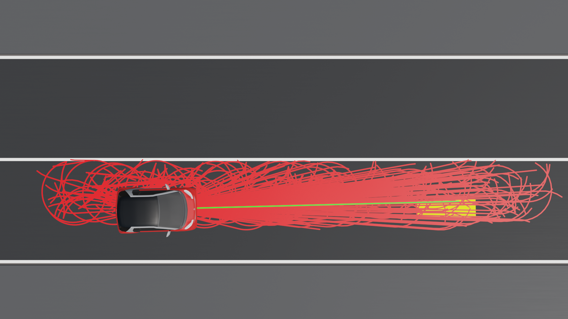
Our goal is to identify the statistical characteristics of the possible occupancy queries generated by a motion planner for a specific task. To achieve this, we define the robot’s task as a set of scenarios, which can also be represented as a distribution of scenarios. Through simulating these scenarios, we collect the generated occupancy queries and store them in a comprehensive database. Systematically gathering these queries allows us to gain a deeper understanding of the perception requirements necessary for the robot to navigate safely and efficiently across all potential situations it may encounter.

For each scenario, we leverage prior knowledge about where obstacles are likely to be. This concept is essential for determining the perception requirements of our autonomous agent. Imagine if vehicles could appear from anywhere—sidewalks, rooftops, or even falling from the sky. Such a scenario would require a comprehensive sensor system capable of monitoring everything. However, by understanding where objects are likely to be, we can strategically position sensors to optimize performance and efficiency. For example, on a highway, we can predict that vehicles will not approach us head-on in our lane. Similarly, for a warehouse robot, we might know that one area is frequented by humans while another is used exclusively by robots. This prior knowledge allows us to refine our perception system, focusing sensor coverage where it is most needed and reducing unnecessary redundancy. By incorporating this knowledge into our design, we can tailor our sensor selection and placement more effectively, ensuring that our autonomous agents are both efficient and well-suited to their specific environments.

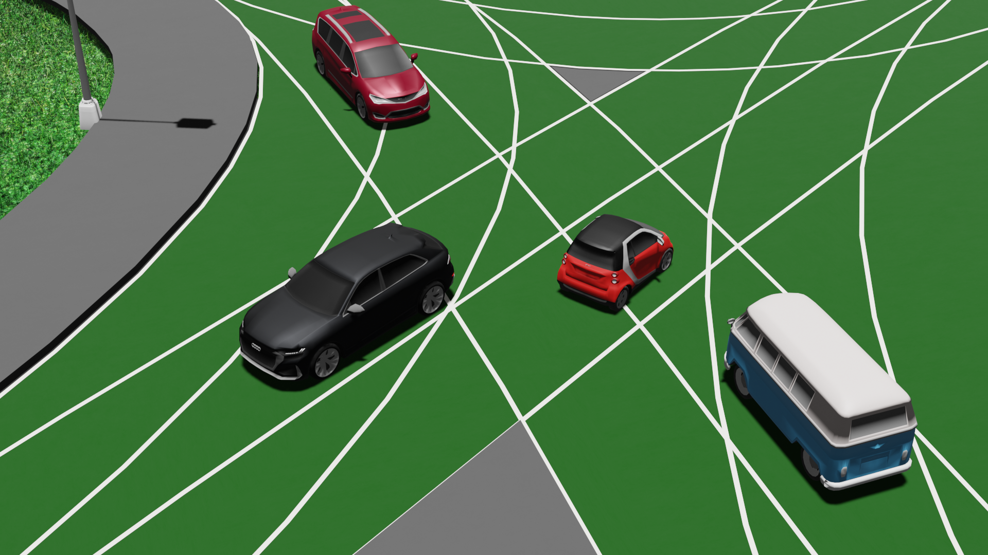
Given our understanding of occupancy queries and our prior knowledge of where objects are likely to be, we can now define the perception requirements for our autonomous vehicle. Consider a small red autonomous vehicle starting from configuration \(q_0\) at time \(t_0\), with the goal of reaching the yellow area.

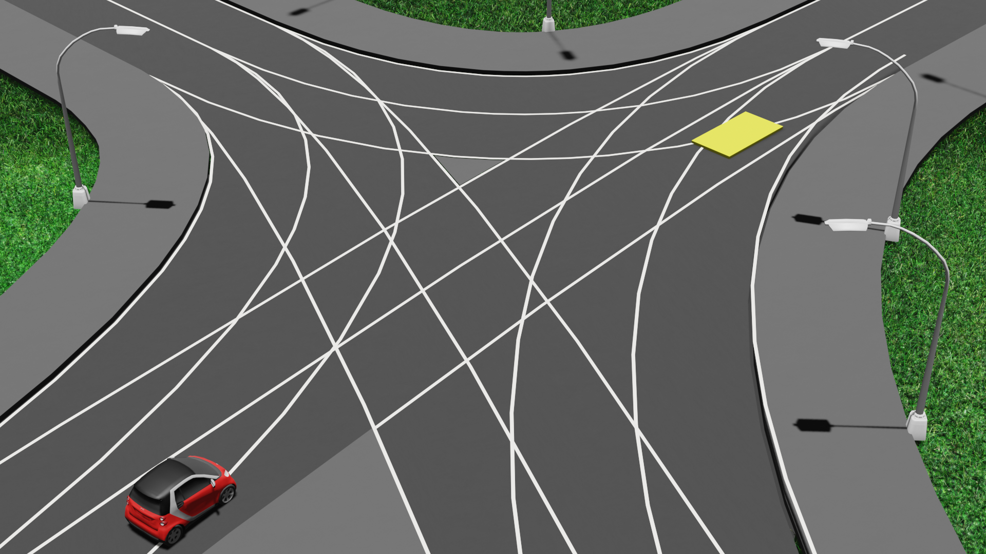
The motion planner generates the following yellow trajectory with an occupancy query at configuration \(q_i\) at a future time step \(t_i\), indicated with the transparent red car. The key question is: where should the sensors focus to accurately respond to this occupancy query?

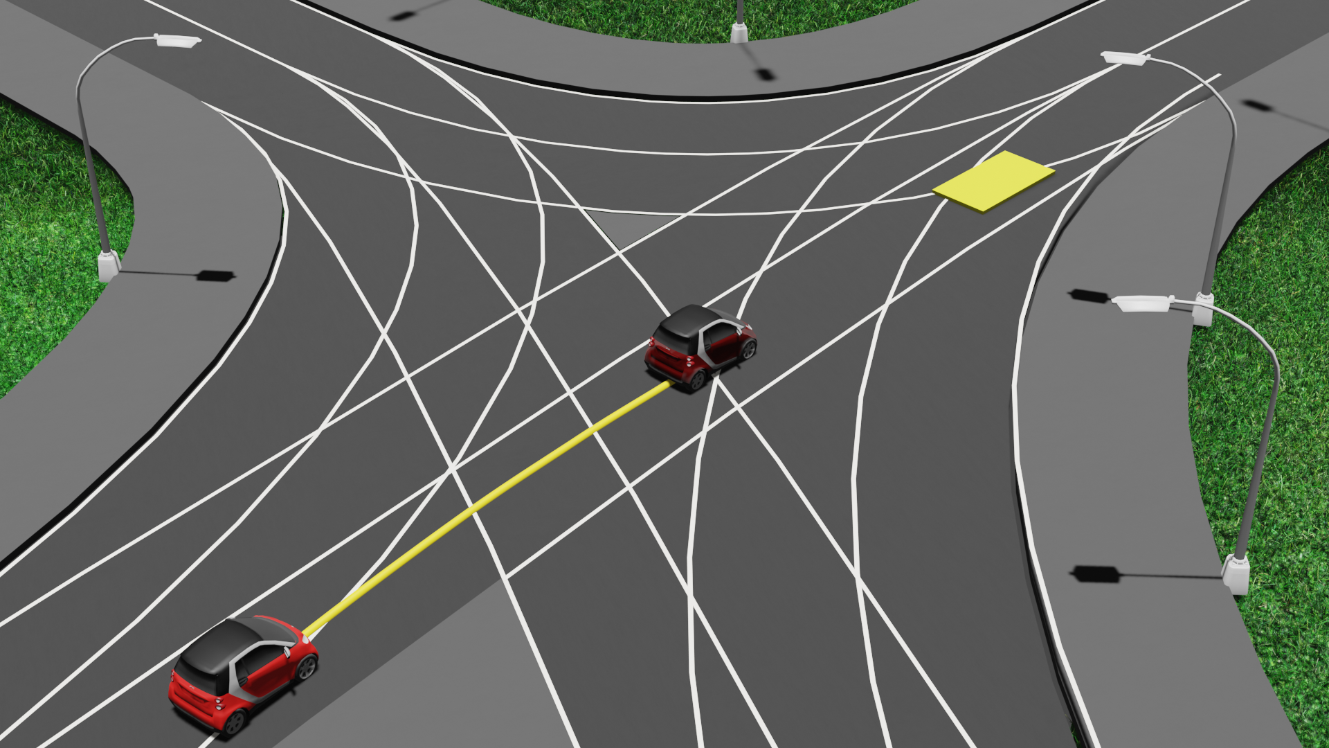
It is similar to how we humans drive. The sensors need to detect all obstacles that could potentially collide with the vehicle at configuration \(q_i\) in the future at time \(t_i\). This involves identifying all possible obstacle trajectories that could lead to a collision at \(t_i\).

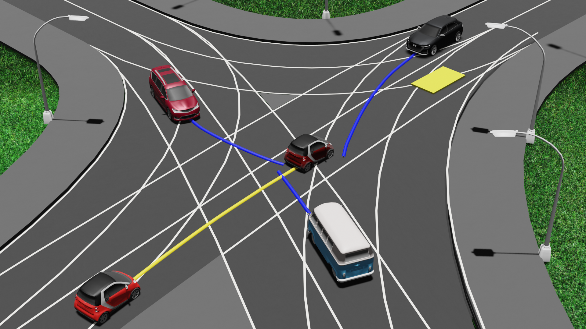
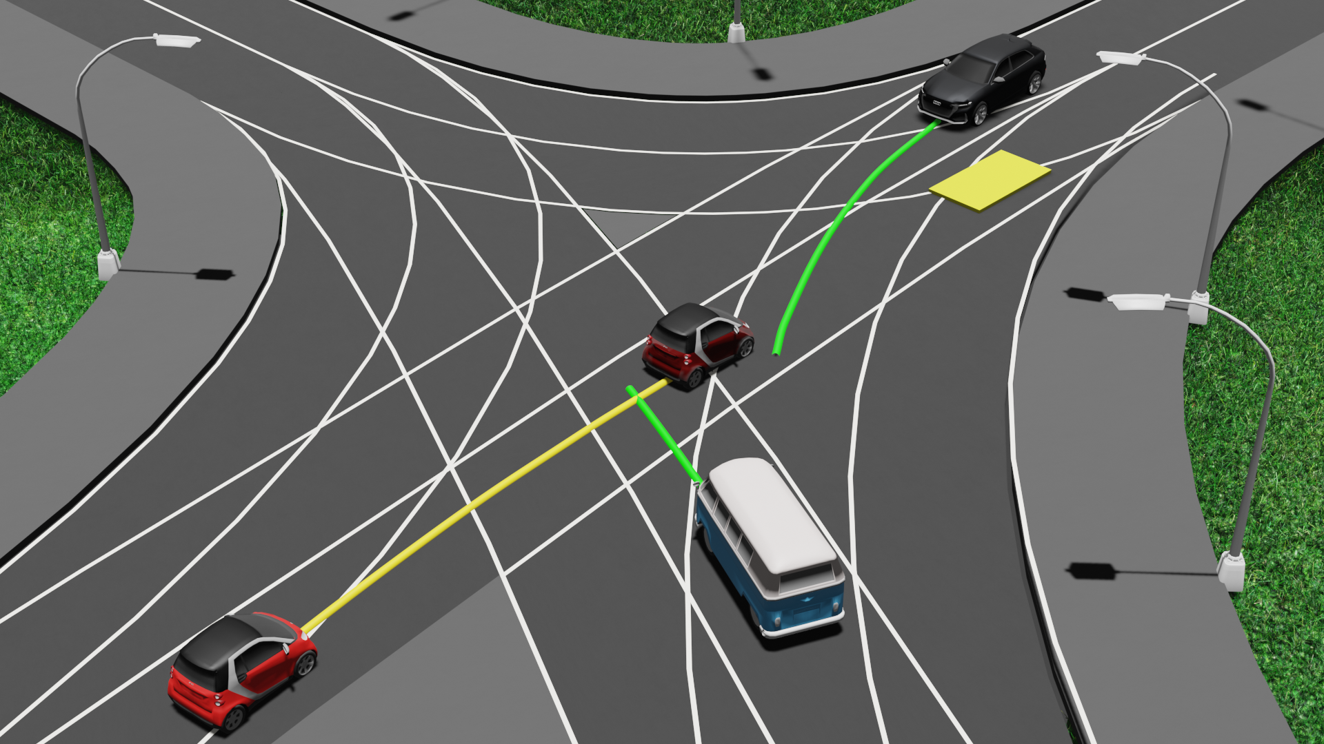
Now, our prior knowledge comes into play. Among the potential trajectories, some may be deemed infeasible based on the prior knowledge. For example, the red car following the red trajectory is known to be infeasible because it is not permitted to turn left. In contrast, the green trajectories are feasible according to our prior knowledge.

Therefore, to answer the motion planner's occupancy query at time \(t_i\), the perception system needs to detect the bus and the black car. By conducting this analysis for all generated occupancy queries related to the robot’s task, we can identify the object configurations that the perception system must be able to detect.

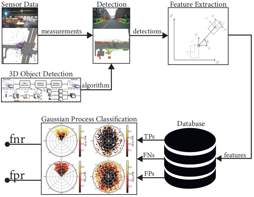
With a clear understanding of the perception requirements for our motion planners, the next crucial step is to benchmark our perception pipelines, which consist of combinations of sensors and their corresponding detection algorithms for processing sensor data. Benchmarking enables us to evaluate how effectively the perception systems deliver the necessary information.

Our perception pipeline benchmarking process follows the following steps: we utilize real sensor data with annotations from the open-source AV dataset, Nuscenes, along with pre-trained perception algorithms from MMDetection3d. We run the inference process to obtain detections, which are categorized as False Negatives (FN), False Positives (FP), and True Positives (TP). From these detections, we extract relevant features, such as the distance of the event relative to the sensor and environmental conditions, and store this data in a database.

Using this data, we perform a binary classification to estimate the False Negative Rate (FNR) and False Positive Rate (FPR):

• FNR: the probability that an object is present but not detected.
• FPR: the probability that a detection is made when no object is present.

For our FNR and FPR models, we also estimate the uncertainty, providing a confidence interval for each estimate. This helps us gauge the model’s confidence in the FNR or FPR values. In our analysis, we adopt a worst-case approach, considering the maximum possible FNR or FPR to ensure that our perception system remains robust and reliable under the most challenging conditions.

Through this benchmarking process, we can assess the performance of our perception pipelines.

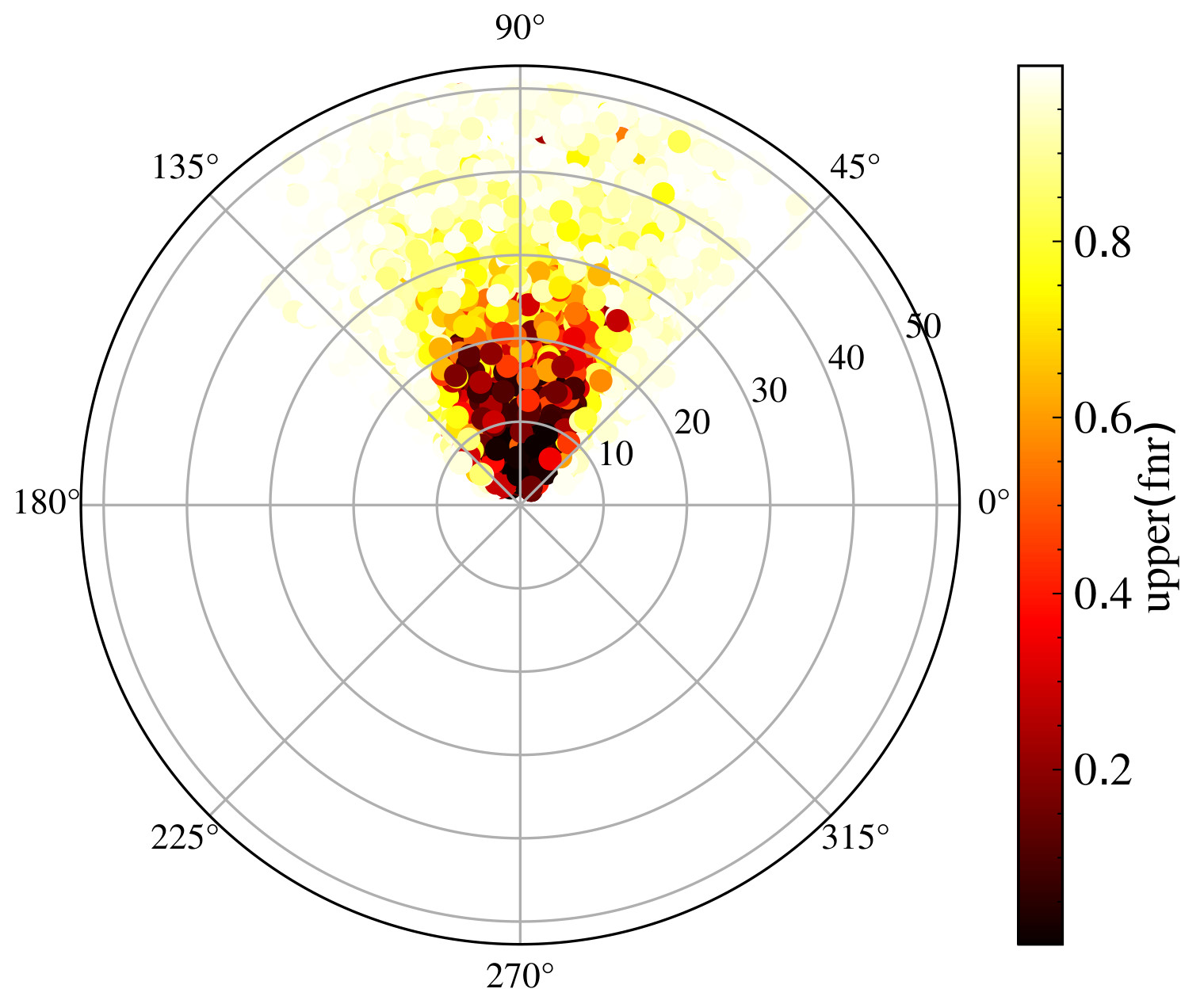
Let's examine some benchmarking results for lidar and camera sensors. On the left, we have a polar plot showing the FNR, and on the right, a plot for the FPR for a perception pipeline using lidar sensors. The points represent object positions relative to the sensor in polar coordinates, with color intensity indicating performance—darker colors represent lower FNR or FPR. We observe that both FNR and FPR increase with distance. This is because fewer lidar points reach distant objects, or the resolution decreases, making them harder to detect accurately. Similar plots are shown for the camera sensor. Unlike lidar, the camera has a limited field of view rather than 360 degrees. As with lidar, performance decreases with distance. Additionally, at the edges of the camera’s field of view, performance drops as objects may only be partially visible. These insights are crucial for understanding the strengths and limitations of each sensor type, allowing us to make informed decisions about sensor placement and usage in our perception system.

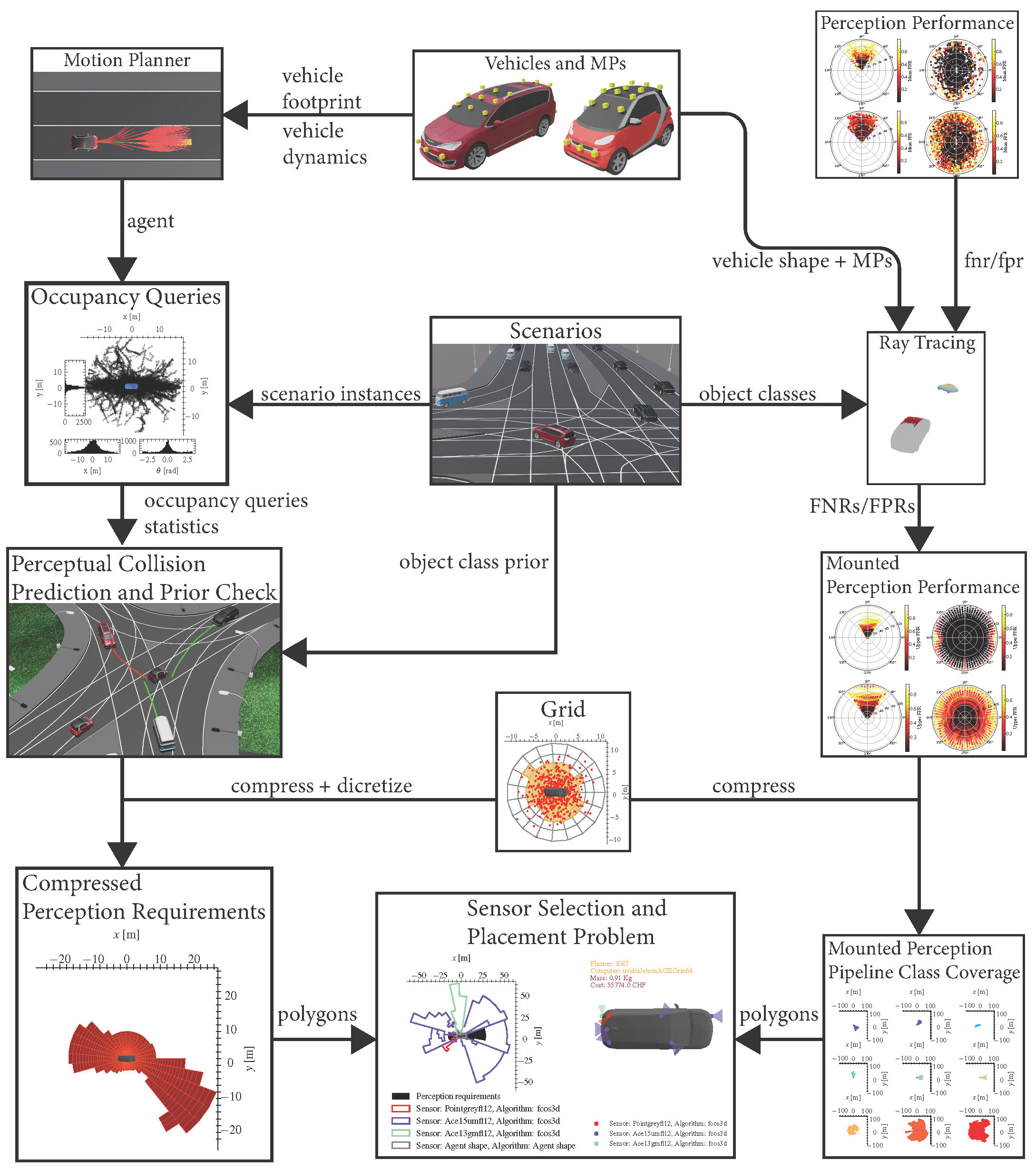
With a method for quantifying the perception requirements for a motion planner and evaluating the performance of various perception pipelines, we can now formulate an optimization problem. The goal of this problem is to identify the perception pipelines that meet the necessary requirements while minimizing resource usage.

We begin by defining the task, represented as a set of scenarios. Next, using predefined vehicle bodies and motion planners, we simulate these scenarios to gather the generated occupancy queries. By integrating our prior knowledge of object configurations with the occupancy queries, we establish the perception requirements. In parallel, we benchmark the perception pipelines, check for occlusions, and evaluate the performance of the mounted sensors. Using a given grid, we compress and discretize both the perception coverage and the perception requirements. Finally, we solve the sensor selection and placement problem as a set cover problem. The result is a set of selected sensors and perception pipelines, including their mounting positions and orientations, that minimize specific costs such as price, mass, power consumption, or computing resources. This approach ensures that our autonomous system is optimized for both performance and efficiency, meeting all necessary perception requirements while minimizing resource usage.

We have explored how to select the optimal perception pipelines for a given task, motion planner, and vehicle. But what if our goal is to find the overall optimal design by also optimizing the vehicle body and motion planner itself?

To achieve an overall optimal design, including vehicle body and motion planner optimization, we leverage the monotone co-design theory developed by Dr. Andrea Censi. For deeper insights into the theory I recommend the reference "Applied Compositional Thinking for Engineers" by Andrea Censi, Jonathan Lorand and Gioele Zardini.

In this approach, the design problem is modeled as a feasibility relation, where functionalities and resources are represented as partially ordered sets. For a detailed reference on partial orders, see Davey and Priestly. This structure allows us to effectively model costs. For example, as in the earlier cleaning robot scenario, we prefer lower prices over higher ones. However, some costs may be incomparable; for instance, one robot may have lower costs but higher mass. Design choices, such as a particular robot design—referred to as implementations—can be mapped to specific functionalities and resources.

Feasibility Relation

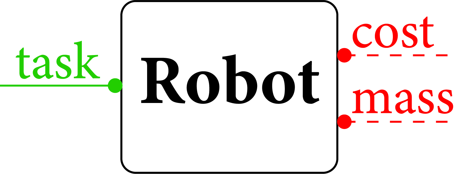
For each design problem, we define a map that identifies the set of implementations for which functionalities \(f\) are feasible with resources \(r\). This is a monotone map, ensuring that requiring fewer functionalities does not demand more resources, and using more resources does not yield fewer functionalities.

This abstract framework can be represented diagrammatically, providing a clear visualization of the design space. How can engineers use this framework? Feasibility relations can be populated in several ways:

• Catalogs: as seen with the cleaning robot example, we use catalogs to compare price and functionalities.
• First Principles: for instance, the energy needed to clean a room is always greater than or equal to the duration of the cleaning process times the power consumption of the robot.
• Data Points: feasibility relations can also be derived from simulations or experiments.

Solving the Optimization Problem

We can solve two types of queries:

• Fixed Functionality Query: we fix the desired functionality and find design solutions that minimize resource usage.
• Fixed Budget Query: we fix a resource budget and find implementations that maximize functionalities.

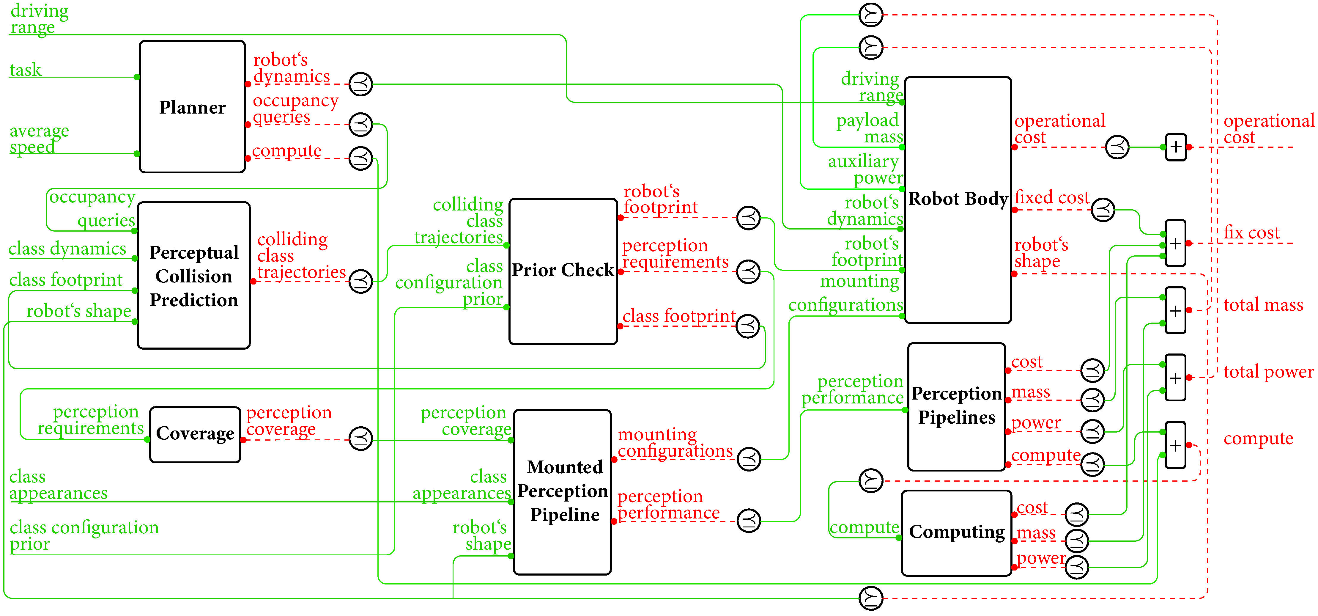
A powerful feature of this tool is its ability to compose and interconnect different design problems. For example, we can arrange design problems in series , in parallel , or even in feedback loops . When two design problems are combined, they form a new, integrated design problem. This flexibility allows us to address complex design challenges by breaking them down into manageable sub-problems, each of which can be optimized individually or in conjunction with others. By leveraging this compositional approach, we can systematically explore the design space, ensuring that our solutions are not only optimal but also robust and adaptable to various scenarios and requirements.

In this case study, we explore the design of an autonomous vehicle using urban driving scenarios from the CommonRoad dataset. These scenarios, derived from real-world maps of various countries, provide a diverse and challenging environment for our vehicle. For object detection, we employ the MMDetection3d library, utilizing PointPillars for lidar and FCOS3D for cameras. For motion planning, we use the OMPL library, a widely used open-source library for sampling-based motion planning algorithms. Specifically, we consider three planners: a lattice planner with A* search, the RRT planner, and the RRT* planner. Our vehicle body options include three types: a small hatchback, a van, and a sedan. To enhance sensing capabilities, we have around ten different sensors, including lidars and cameras with various resolutions and specifications. Additionally, we have a selection of ten computers with varying levels of computing power. It is important to note that designers are free to generate their own catalogs of software and hardware components.

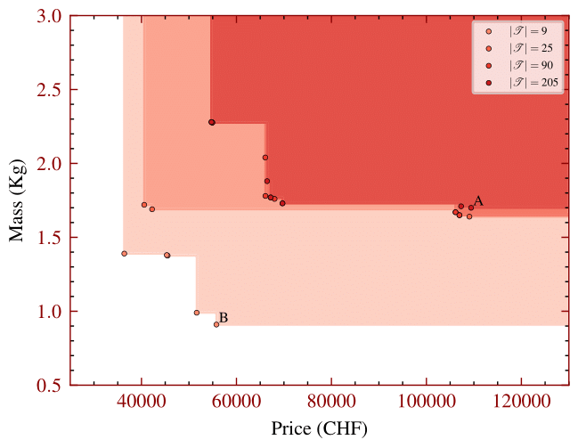
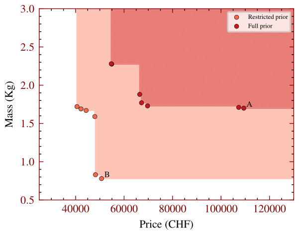
Let's explore how the number of scenarios in a task impacts resource usage in the design of our autonomous vehicle. More scenarios generally require more resources, as demonstrated in the following series of plots. The first plot shows Pareto fronts comparing the total mass (in kilograms) of selected sensors and computers against the total cost (in Swiss francs). Different shades of red represent varying numbers of scenarios:

• Dark red: 205 scenarios.
• Brightest red: 9 scenarios.

Each point represents an optimal solution, and the red area highlights the feasible resource range, indicating that similar solutions may demand more resources as the task complexity increases. The design choices with the lowest mass for the maximum and minimum tasks are also shown. Triangles represent the orientation of cameras, while squares represent lidars, with the same perception pipeline color-coded. Cameras are prioritized due to their lighter weight compared to lidars. The most powerful computing unit is required because camera-based perception algorithms, which typically involve large neural networks with more parameters, demand higher computational power.

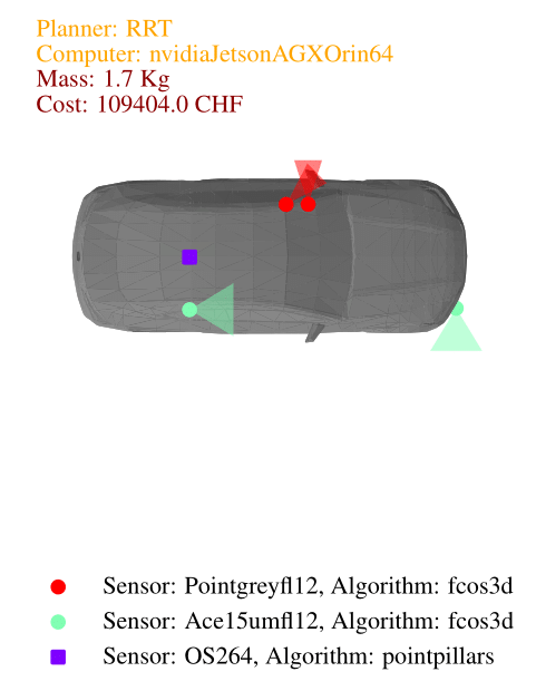
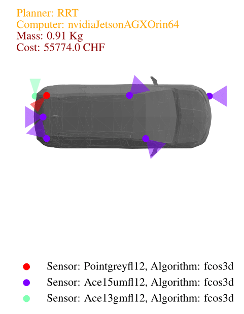
Nominal speed in scenarios has a significant impact on resource usage. Higher nominal speeds require more resources for several reasons:

• Motion planners generate longer-range trajectories.
• Sensors need to cover a greater range to detect objects at higher speeds.

The following plot shows the Pareto fronts for total power consumption of the selected sensors and computing units (in watts) and total cost (in Swiss francs) for different nominal speeds. The plot demonstrates how increasing nominal speed demands additional resources.

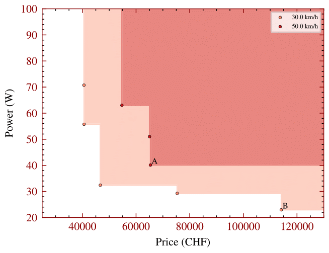
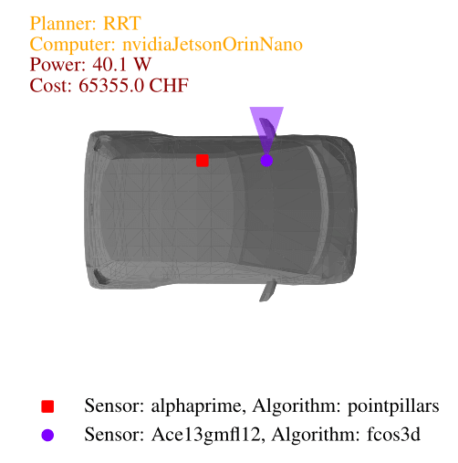
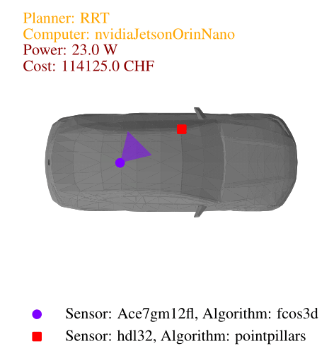
Prior knowledge of where objects can be located in scenarios also influences resource consumption. More potential object positions increase perception requirements, demanding additional or higher-quality sensors and perception algorithms. In this study, we restricted the prior knowledge, preventing vehicles from approaching from the left or behind. This illustrates how limiting possible object positions can reduce resource needs.

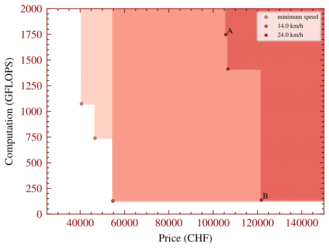
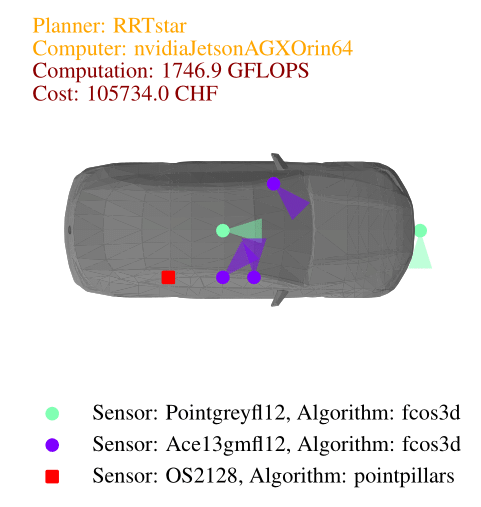
When solving the co-design problem, we can fix certain functionalities and identify implementations that minimize resource usage. In this case, we explore the impact of requiring higher task performance, specifically a higher average speed. For higher average speeds, the results show that the only asymptotically stable motion planner, RRT*, is necessary, along with the vehicle body offering the highest acceleration—the sedan. In the image below we show the Pareto fronts for total computation needed by the perception and planning algorithms (in GFLOPS) and total cost (in Swiss francs) for different average speeds. From the implementation plots we can see that cameras are generally cheaper than lidars, making them the preferred choice in the least expensive designs.

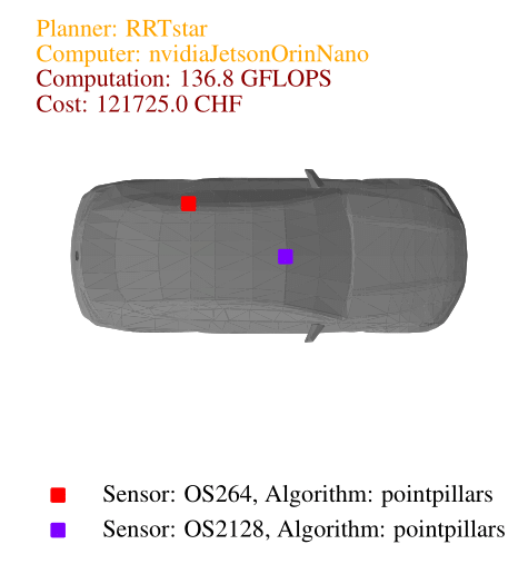
Conclusion

• Higher average speeds require more sophisticated motion planners and vehicle bodies with better dynamics.
• Cameras are favored in designs prioritizing lower mass and cost.
• Lidars are preferred when minimizing computational resources.
• Overall, lidars are more powerful and are always selected for the most complex tasks.